Introduction to NumPy
In a world without NumPy
NumPy is gold. In a world without a numeric library like Numpy, this age of Artificial Intelligence wouldn’t exist as we would not have been able to train Machine Learning algorithms.
Simple addition of two lists without NumPy -
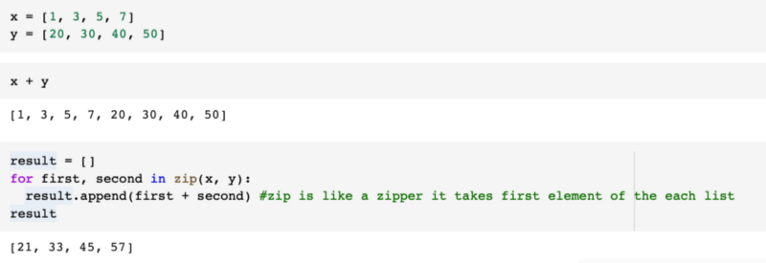
You can anticipate that if we have a lot of data or a multi-dimensional value, we will require two or more layers of for loop, which will slow down computation.
About NumPy — see the light!
NumPy deservedly bills itself as the fundamental package for scientific computing with Python.

NumPy is a module for Python. The name is an acronym for “Numeric Python” or “Numerical Python”.
NumPy is a merger of two Python modules, it is mostly written in C. Numeric is like NumPy, a Python module for high-performance, numeric computing. Numarray, is a complete rewrite of Numeric but is now deprecated.
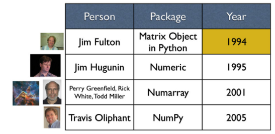
Jim Hugunin wrote Numeric (Numerical Python) in 1995 with help from a bunch of other people, and Travis Oliphant.
In 2005, Travis Oliphant created NumPy by incorporating features of the competing Numarray into Numeric.
Core Python vs NumPy with Python
Python was not originally intended for numerical computing. The demand for quick numeric calculation developed as individuals began to use Python for diverse tasks
The advantages of Core Python:
- It has high-level number objects: integers, floating point
- containers: lists with cheap insertion and append methods, dictionaries with fast lookup.
Advantages of using NumPy with Python:
- It does array oriented computing
- It efficiently implements multi-dimensional arrays
- It is designed for scientific computation
Python list vs Python array
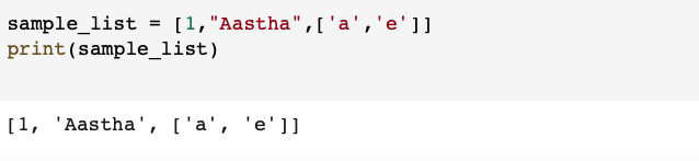
A list in Python is a collection of items which can contain elements of multiple data types, which may be either numeric, character logical values, etc.
- It cannot directly handle arithmetic operations.
- It’s flexibility allows easy modification (addition, deletion) of data.
- The entire list can be printed without any explicit looping.
An array is a vector containing homogeneous elements allocated with contiguous memory locations allowing easy modification.
- Can directly handle arithmetic operations.
- Less flexibility since addition, deletion has to be done element wise.
- A loop has to be formed to print or access the components of array.

Built-in array vs NumPy array
Built-in array : The objects stored in the array are of a same type and is determined by typecode. Type codes are single characters.
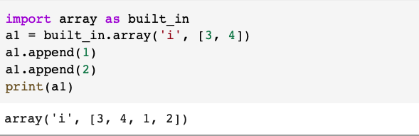
- Built-in array module does not typecast data implicitly (example : if here we provide a float input, it will give us a TypeError as it from float to int)
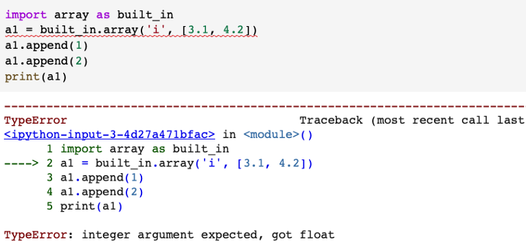
Typecode ‘i’ indicates , objects stored in the array must be of ‘int’ type. Trying to store floating-point value, caused a TypeError.
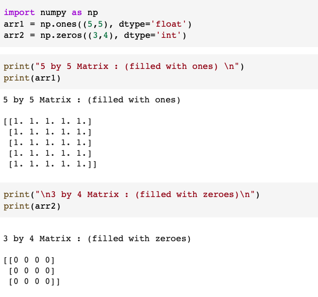
NumPy array: NumPy module in python is generally used for matrix and array computations.
Using the NumPy module, built-in function ‘array’ is used to create an array.
- NumPy array is flexible in the matter of typecasting, it will upcast or downcast and try to store the data at any cost. (Float was converted to int, even if that resulted in loss of data after decimal)
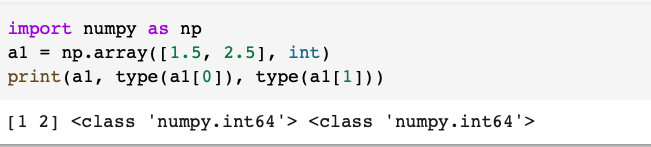
Here floating point data was typecasted into int
Python list vs NumPy array - since 2005

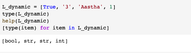
- The Python core library provided Lists. A list is a collection of data type that can be of homogeneous or heterogeneous.
- NumPy array is a grid of orderly allocated values of the homogeneous data types. Element wise operation is possible.
If You Want To Get Ahead, Get a Speed of NumPy!
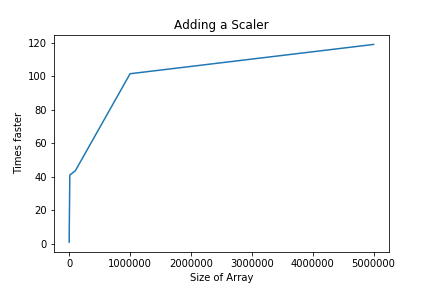
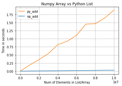
How fast is Numpy?
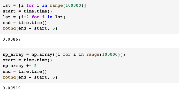
Numpy array performs 5 times faster than Python List for Scalar Addition
Why is it so fast?
-
Memory Consumption
Numpy arrays store one defined type of data as one contiguous block of memory.

Array in RAM
With the array’s initial memory address known, we can simply add the index to jump to any element.
Python lists are actually arrays of pointers. A pointer is a reference to an object in memory.
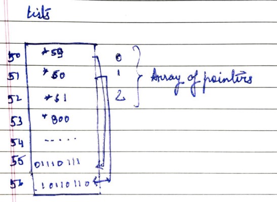
List’s memory allocation
Python takes two steps when retrieving the first entry in your list which decreases performance: Obtain the pointer first. Second, go to the pointer’s memory address to retrieve the object.
-
Computation process
-
Numpy is able to divide a task into multiple subtasks and process them.
-
NumPy combines C, C++, and Fortran code. In comparison to Python, these programming languages have an extremely short execution time.
-
Why does speed matter?
The small differences in runtime become amplified with repeated function calls, which cumulates to a large inference time hence slower computation.
-
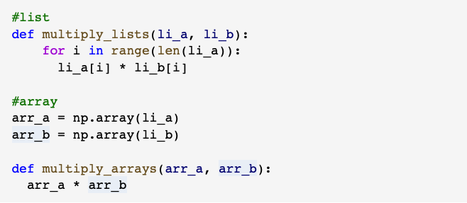
We understand now that Loops slow our code! So, let’s write a code that takes two arrays and performs element-wise multiplication.
-
if we are using NumPy arrays, we do not need to write a loop. We can simply do this like shown below.
Preparing multiplication of lists and the NumPy arrays
- When using the NumPy’s solution, there are significant speedups of nearly 20–30 times.
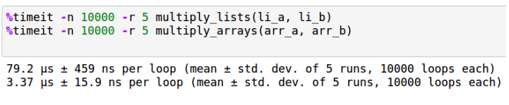
It took 79 μs for a loop to multiply list, whereas 3.4 μs to multiply NumPy array
Limitation of vectorization - It can be only be done on a loop which performs operations on two arrays of equal size or between an array and a scalar.
What happens if we want to vectorize a loop that involves arrays of different sizes?
Method 1: To loop over the columns of matrix, and add each columns.
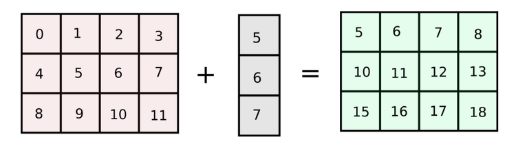
Addition matrix of shape (3,4) and column vector
Drawback: Since we are looping, the code described above will execute slowly if the number of columns in the original array gets increased to a large number.
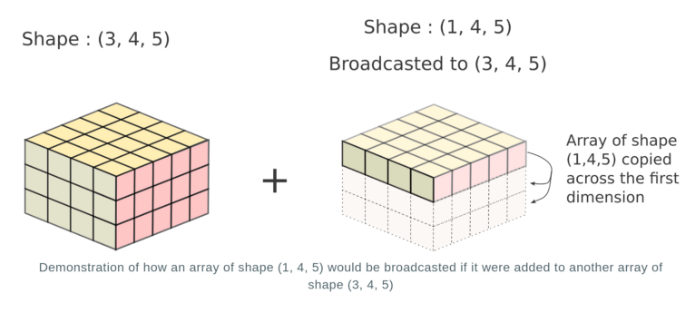
Method 2: Make a matrix of the same number of columns as the original array.
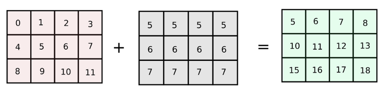
This gives us a much faster solution. This important NumPy abstraction is called Broadcasting.
“Subject to certain constraints, the smaller array is “broadcast” across the larger array so that they have compatible shapes. Broadcasting provides a means of vectorizing array operations so that looping occurs in C instead of Python”
NumPy to its full capacity!
This blog will now also show you how to utilise NumPy to its best potential by exhibiting how to use Vectorization and Broadcasting.
Understanding Rules for Broadcasting
NumPy’s broadcasting rule relaxes this constraint when the arrays’ shapes meet certain constraints.
Addition matrix of shape (3,4) and column vector
For just two arrays, NumPy compares the shape of the two arrays dimension-by-dimension starting from the trailing dimensions of the arrays working it’s way forward. (from right to left)
Two dimensions are compatible when:
- Dimensions are equal
- One of them is 1
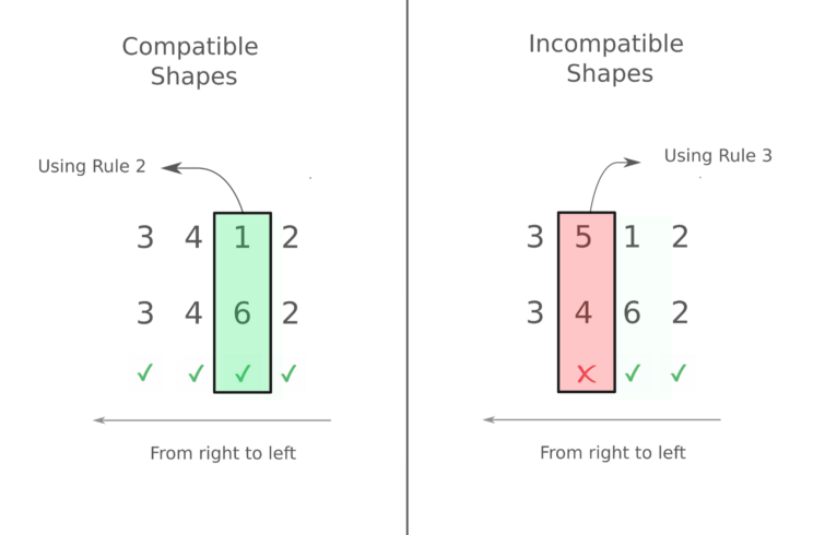
Equal Ranks and equal values
In case of example on the right, starting from left, when we arrive at the 2nd dimension, there’s a difference and neither of them is 1. Therefore, trying to do an operation with them leads to an error.
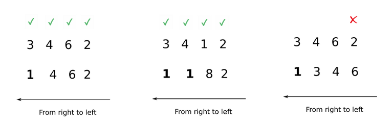
Unequal ranks
In order to compare two such arrays, Numpy appends dimensions of size 1 to the smaller array so that it has a rank equal to the larger array to make it compatible.
Conclusion
Woo Hoo! Congrats for making it all the way to the end of this blog. Thank you very much for taking the time to read this. Despite the fact that it was only a tooth in NumPy’s gear wheel, I hope it was useful in getting you up and going.
Did you like NumPy’s superpowers? Please let me know in the comments section where all thoughts and insights are eagerly appreciated.
Stay tuned for the next blog in which we will continue exploring and learning NumPy by delving deeper into its features such as broadcasting, vectorization, indexing, ufunc and Numba as well as how they help in real world scenarios.